 Fireblaze
Learning Guides
Excel Formulas With IF Condition, VLOOKUP and XLOOKUP: When to Use Which
Excel formulas with IF condition, VLOOKUP and XLOOKUP explained with tested examples, the 5 errors that break lookups, and a free practice workbook.

You know IF exists. You have probably copied a VLOOKUP from a colleague's file. But when a new task lands, you still stop and wonder which one you actually need.
This guide fixes that. You will learn how Excel formulas with an IF condition work, how VLOOKUP and XLOOKUP fetch data, and a simple three-question test for choosing between them.
The examples all use one practice workbook, which you can download below. It includes the five mistakes that quietly return wrong numbers.
An Excel formula with an IF condition tests whether something is true and returns one result if it is and another if it isn't, for example =IF(B2>=40,"Pass","Fail"). VLOOKUP and XLOOKUP do a different job: they find a value in a table, such as a product code, and return related data like its price.
Quick answer: Excel formulas with IF condition vs VLOOKUP vs XLOOKUP (November 2026)
- Use IF when you are deciding something from a rule, like
=IF(B2>=40,"Pass","Fail"). Add AND or OR when the rule has two conditions.- Use IFS or a slab table instead of nested IF once you have more than three rules. IFS is available in Excel 2019 and later and accepts up to 127 conditions.
- Use VLOOKUP when the file must open in Excel 2019 or older, and always type FALSE as the fourth argument for an exact match.
- Use XLOOKUP in Microsoft 365, Excel 2021, Excel 2024 and Google Sheets. It defaults to an exact match, can look left and has a built-in "not found" message.
- In our practice workbook, leaving out VLOOKUP's fourth argument gave a wrong price on 4 of 8 orders without showing a single error.

About the Practice Workbook
All examples use one small workbook: a fictional Nagpur electronics store with 8 products, 8 orders, 6 sales staff and a commission slab table. You can download it in the practice section and follow along.
How we tested: the IF, AND, IFS, TRIM, IFNA, INDEX-MATCH and VLOOKUP results were recalculated in LibreOffice Calc 24.2 on 19 November 2026. LibreOffice 24.2 does not support XLOOKUP, so every XLOOKUP example in this guide follows Microsoft's documented behaviour. To see those cells calculate, open the workbook in Microsoft 365, Excel 2021 or Excel 2024.
Excel Formulas With IF Condition: The Basics
The IF function checks one condition and returns one value when it is TRUE and another when it is FALSE. Microsoft documents the syntax as IF(logical_test, value_if_true, [value_if_false]) on its IF function support page.
The three parts:
- logical_test: the question, such as
B2>=40orC2="Nagpur". - value_if_true: what to show if the answer is yes.
- value_if_false: what to show if the answer is no.
Three examples you can type right now:
| Task | Formula | Result |
|---|---|---|
| Mark pass or fail | =IF(B2>=40,"Pass","Fail") | Pass if B2 is 40 or more |
| Flag over budget | =IF(C2>D2,"Over budget","OK") | Over budget if spend beats budget |
| Calculate a bonus | =IF(B2>=100000,B2*5%,0) | 5% of sales, or 0 |
Two rules trip up beginners:
- Text goes inside double quotes. Numbers never need them.
- Comparison operators are
=,<>(not equal),>,<,>=and<=. Type>=with no space.
Pro tip: press Ctrl + ` to switch every cell from results to formulas. It is the fastest way to audit someone else's sheet.
Excel Formulas With IF Condition and Multiple Rules (AND, OR)
Wrap AND or OR inside IF when one decision depends on two or more conditions. AND returns TRUE only if every condition is true. OR returns TRUE if any one of them is.
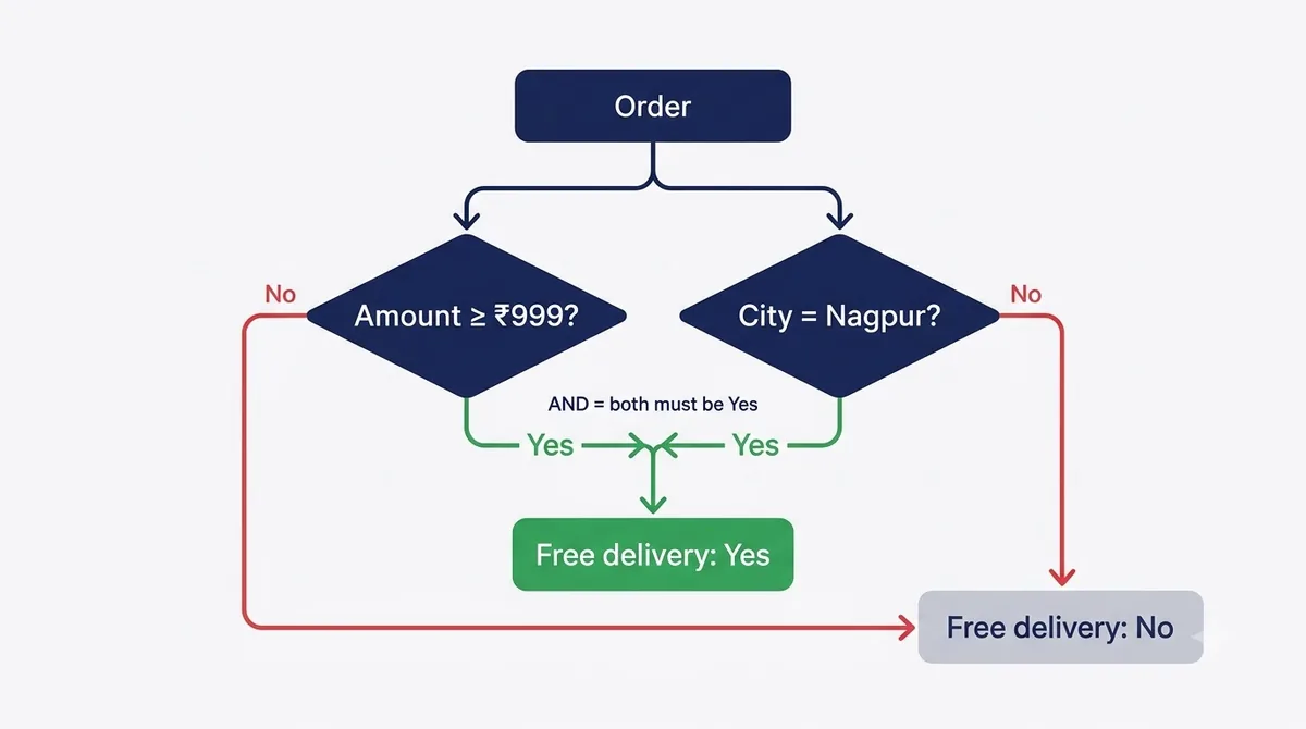
In our workbook, the store gives free delivery only to Nagpur orders of ₹999 or more. That is an IF with AND:
=IF(AND(G2>=999, B2="Nagpur"), "Yes", "No")Result on our 8 orders: 2 got "Yes", the ₹10,499 monitor and the ₹2,199 webcam, both Nagpur orders. The ₹2,697 Amravati order got "No" because it failed the city test. The ₹499 Nagpur pen drive got "No" because it failed the amount test.
Swap in OR when either condition is enough:
=IF(OR(B2="Nagpur", G2>=5000), "Free delivery", "Charge ₹99")Excel text comparisons ignore case, so "nagpur" matches "Nagpur". Extra spaces are not ignored, as the mistakes section shows.
Nested IF vs IFS Function vs a Slab Table
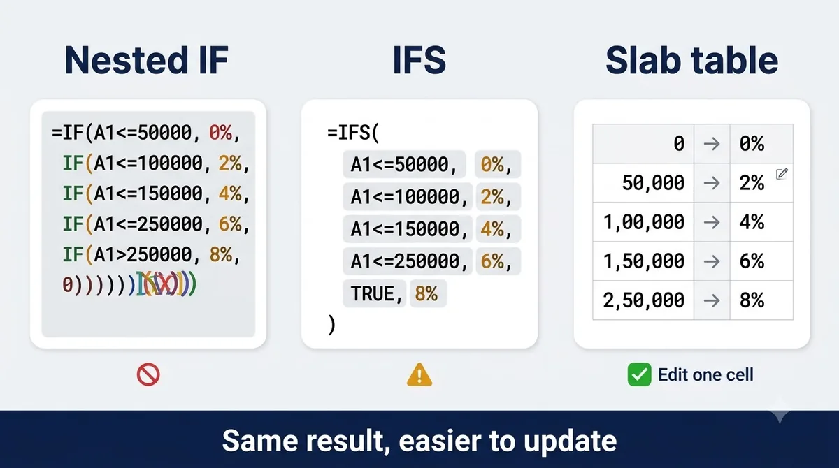
A nested IF puts one IF inside another to test several conditions in order. Once you pass three or four rules, IFS or a lookup slab table is easier to read and safer to edit.
We tested all three methods on the same commission rule: 0% below ₹50,000, then 2%, 4%, 6% and 8% from ₹2,50,000.
Method 1: Nested IF (works in every Excel version)
=IF(B2>=250000,8%,IF(B2>=150000,6%,IF(B2>=100000,4%,IF(B2>=50000,2%,0))))Method 2: IFS (Excel 2019 and later)
=IFS(B2>=250000,8%,B2>=150000,6%,B2>=100000,4%,B2>=50000,2%,TRUE,0)Microsoft's IFS page says IFS can test up to 127 conditions. The final TRUE,0 acts as "everything else". Without it, IFS returns #N/A when no rule matches.
Method 3: Slab table with approximate VLOOKUP
Put the slabs in two columns (0, 50,000, 1,00,000, 1,50,000, 2,50,000 and their rates), sorted smallest first. Then:
=VLOOKUP(B2, $H$2:$I$6, 2, TRUE)All three methods returned identical rates for our six staff:
| Staff | Monthly sales | Nested IF | IFS | Slab VLOOKUP |
|---|---|---|---|---|
| Aarti | ₹42,000 | 0% | 0% | 0% |
| Rohit | ₹98,000 | 2% | 2% | 2% |
| Pooja | ₹99,999 | 2% | 2% | 2% |
| Sneha | ₹1,50,000 | 6% | 6% | 6% |
| Kunal | ₹2,00,000 | 6% | 6% | 6% |
| Imran | ₹2,75,000 | 8% | 8% | 8% |
Notice Pooja at ₹99,999: one rupee short of the 4% slab. Boundary values like this are where hand-typed nested IFs usually go wrong, so test them first.
Which to pick? When the rates change, the slab table needs one cell edited. The nested IF needs every copy of the formula rewritten. For anything that changes, such as commission, tax bands, discount tiers or grade cut-offs, use the table.
Excel Formulas VLOOKUP: How It Works
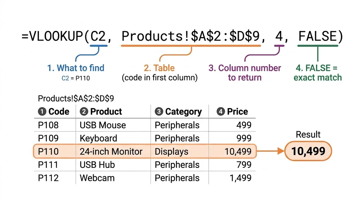
VLOOKUP searches the first column of a table for a value and returns data from a column you specify in the same row. The syntax is VLOOKUP(lookup_value, table_array, col_index_num, [range_lookup]), as shown on Microsoft's VLOOKUP page.
Here is a VLOOKUP example from our orders sheet. It fetches a product's price:
=VLOOKUP(C2, Products!$A$2:$D$9, 4, FALSE)Read it as: "Find the code in C2, in the first column of A2:D9 on the Products sheet, and return column 4 (Price). Exact match only."
| Argument | In our formula | What it means |
|---|---|---|
| lookup_value | C2 | The code to find, e.g. P110 |
| table_array | Products!$A$2:$D$9 | The table, with the code in its first column |
| col_index_num | 4 | Return the 4th column of that table |
| range_lookup | FALSE | Exact match only |
For order FB-1001 (code P110), it returns ₹10,499.
The one rule that matters most: always type FALSE (or 0) as the fourth argument. If you leave it out, VLOOKUP assumes an approximate match, which only works when the first column is sorted. Our product codes are not sorted, and the mistakes section shows what happens.
Also lock the table with $ signs (press F4 after selecting the range). Otherwise the range slides as you copy the formula down, and later rows can return #N/A.
How to Use XLOOKUP in Excel
XLOOKUP searches one column (or row) and returns the matching item from another. It uses exact match by default and can show a message when nothing is found. The syntax is XLOOKUP(lookup_value, lookup_array, return_array, [if_not_found], [match_mode], [search_mode]).
The same price lookup in XLOOKUP:
=XLOOKUP(C2, Products!$A$2:$A$9, Products!$D$2:$D$9, "Not in list")You point at two columns instead of counting them. There is no column number and no FALSE, and the "Not in list" message replaces #N/A.
Availability matters in India, where many offices still use older versions of Excel. Microsoft's XLOOKUP page states that XLOOKUP is not available in Excel 2016 and Excel 2019. It works in Microsoft 365, Excel 2021 and Excel 2024. Google Sheets also supports XLOOKUP.
If you open an XLOOKUP file in Excel 2019, the cells show #NAME?. That is the main reason VLOOKUP is still worth learning.
The optional arguments, per Microsoft's documentation:
| Argument | Values | Use it for |
|---|---|---|
| if_not_found | Any text or value | A friendly message instead of #N/A |
| match_mode | 0 exact (default), -1 exact or next smaller, 1 exact or next larger, 2 wildcard | Slabs and partial text matches |
| search_mode | 1 first to last (default), -1 last to first, 2 and -2 binary search | Finding the latest entry |
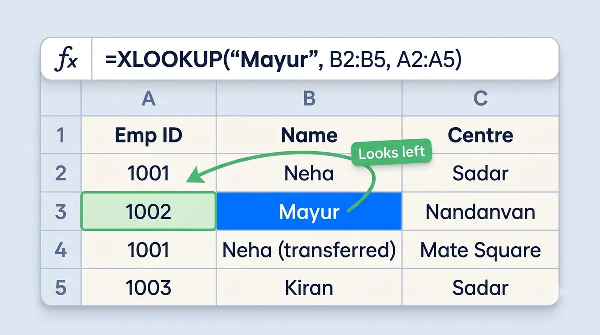
Two things VLOOKUP cannot do:
- Look left.
=XLOOKUP("Mayur", B2:B5, A2:A5)returns Mayur's employee ID (1002), even though the IDs sit to the left of the names. - Get the last match. Employee 1001 appears twice because Neha transferred centres.
=XLOOKUP(1001, A2:A5, C2:C5, , 0, -1)searches from the bottom up and returns her latest centre, Mate Square. VLOOKUP always returns the first row, Sadar.
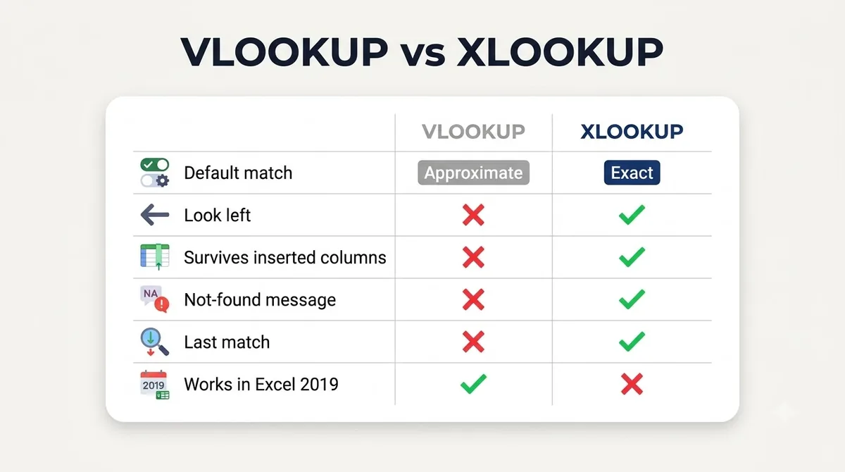
VLOOKUP vs XLOOKUP: Side-by-Side
XLOOKUP does everything VLOOKUP does, with safer defaults. VLOOKUP still wins when a file must work in Excel 2019 or older.
| Feature | VLOOKUP | XLOOKUP |
|---|---|---|
| Default match | Approximate (if the 4th argument is omitted) | Exact |
| Look to the left | No | Yes |
| Survives inserted columns | No (the column number is fixed) | Yes (the return column is a range) |
| Built-in "not found" message | No, wrap it in IFNA or IFERROR | Yes, 4th argument |
| Last match | No | Yes, search_mode -1 |
Wildcards (*, ?) | Yes, in exact match mode | Only with match_mode 2 |
| Return several columns at once | No | Yes |
| Excel 2016 and 2019 | Yes | No |
| Microsoft 365, Excel 2021, Excel 2024, Google Sheets | Yes | Yes |
The wildcard row surprises people. In our Gotchas sheet, =VLOOKUP("Ne*", B2:C5, 2, FALSE) returns Sadar, Neha's centre, because the asterisk matches any text. XLOOKUP ignores wildcards unless you set match_mode to 2.
A VLOOKUP returns only the first match it finds. A SQL join returns every matching row, which is why the two tools can give different totals. Our joins in SQL guide covers that difference.
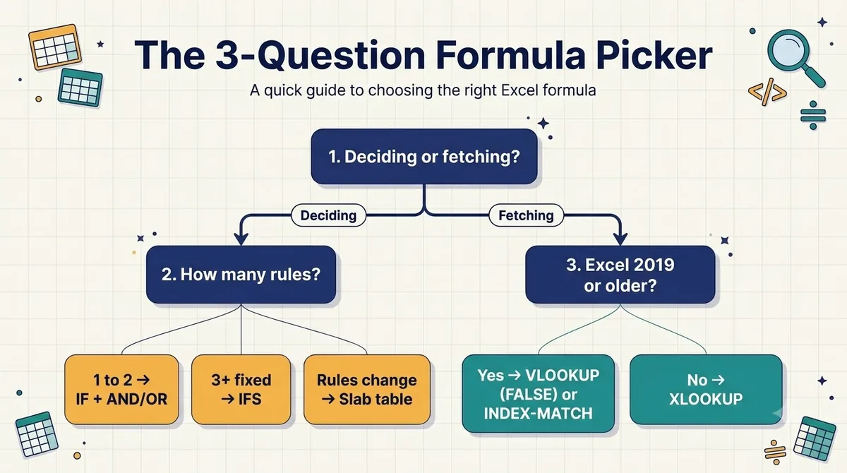
The 3-Question Formula Picker
The 3-Question Formula Picker is a quick test for choosing between IF, IFS, VLOOKUP and XLOOKUP. Decide whether you are applying a rule or fetching data, then check how many rules there are, or which Excel versions will open the file.
Question 1: Am I deciding or fetching?
- Deciding means applying a rule to a value: pass or fail, bonus or no bonus, late or on time. That is the IF family.
- Fetching means pulling data that already exists in another table: price, name, department, rate. That is a lookup.
Question 2 (if deciding): How many rules?
- One or two conditions:
IF, withANDorOR. - Three or more fixed rules:
IFS(Excel 2019 and later) or nested IF. - Rules that will change, such as slabs, bands or tiers: a slab table with
XLOOKUP(..., match_mode -1)orVLOOKUP(..., TRUE).
Question 3 (if fetching): Will anyone open this in Excel 2019 or older?
- Yes, or you are not sure:
VLOOKUPwith FALSE, orINDEXwithMATCHif you need to look left. - No, everyone uses Microsoft 365, Excel 2021 or later, or Google Sheets:
XLOOKUP.
Most office tasks are answered after two questions.
5 Mistakes That Break Lookups (Tested)
Most broken lookups come from five causes: a missing fourth argument, inserted columns, stray spaces, numbers stored as text and duplicate keys. We reproduced each one in the practice workbook.
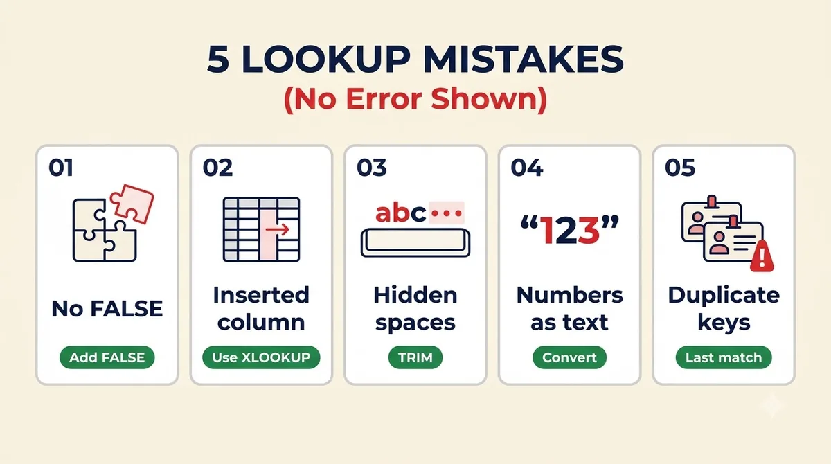
1. Leaving out VLOOKUP's fourth argument
We ran =VLOOKUP(C2, Products!$A$2:$D$9, 4), with no FALSE, next to the correct formula on all 8 orders:
| Order | Code | Correct price | Price with no 4th argument |
|---|---|---|---|
| FB-1001 | P110 | ₹10,499 | ₹10,499 |
| FB-1003 | P103 | ₹499 | ₹2,799 (wrong) |
| FB-1004 | P109 | ₹6,999 | ₹649 (wrong) |
| FB-1007 | "P104 " (trailing space) | #N/A | ₹649 (wrong) |
| FB-1008 | P120 (not in the list) | #N/A | ₹499 (wrong) |
Four of eight orders came back with a wrong price, and not one showed an error. P120 is not in the product list, yet it still got a price. That is why this mistake is so dangerous: the sheet looks fine.
Fix: always add FALSE. XLOOKUP avoids this by defaulting to an exact match.
2. Inserting a column into the lookup table
We added a "Brand" column before Price. The old formula, =VLOOKUP("P110",$A$2:$E$9,4,FALSE), then returned "Displays", the category, instead of ₹10,499, because column 4 is no longer Price.
Fix: point at the Price column directly. =INDEX($E$2:$E$9, MATCH("P110", $A$2:$A$9, 0)) still returned ₹10,499 after the insert. XLOOKUP works the same way because it names the return column rather than counting to it.
3. Hidden spaces
Order FB-1007 was typed as "P104 " with a trailing space. The exact-match VLOOKUP returned #N/A, even though P104 is in the list.
Fix: wrap the lookup value in TRIM. =IFNA(VLOOKUP(TRIM(C8), Products!$A$2:$D$9, 4, FALSE), "Not in list") returns the correct ₹899, and the genuinely missing P120 shows "Not in list".
4. Numbers stored as text
Employee 1003 was saved as text ("1003") in our staff list. Looking up the number 1003 returned #N/A, while looking up the text "1003" found Kiran.
Fix: convert the column with Data, Text to Columns, Finish. Data exported from billing or HR software often arrives as text.
5. Duplicate keys
Employee 1001 appears twice. VLOOKUP returned the first row (Sadar), not the latest (Mate Square). There was no error, just an outdated answer.
Fix: remove duplicates first, or use XLOOKUP with search_mode -1 to get the last match. To find duplicates before you look up, use =COUNTIF(A:A, A2)>1.
Excel Formulas With IF Condition Plus VLOOKUP or XLOOKUP
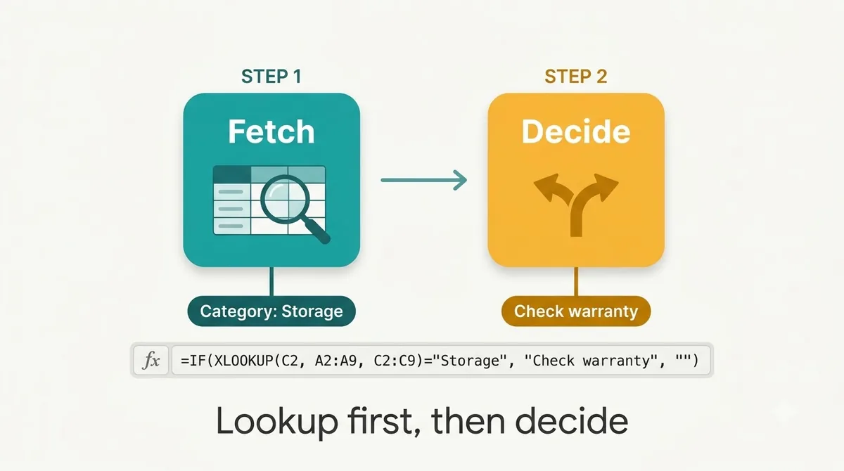
IF and lookups work best together: the lookup fetches a value, and IF decides what to do with it. Three patterns cover most office work.
1. Hide errors with a message (IFNA)
=IFNA(VLOOKUP(C2, Products!$A$2:$D$9, 4, FALSE), "Not in list")Prefer IFNA over IFERROR for lookups. IFERROR also hides mistakes such as a wrong sheet name, so a broken formula looks like a missing product.
2. Decide based on a fetched value
=IF(XLOOKUP(C2, Products!A2:A9, Products!C2:C9)="Storage", "Check warranty", "")This flags every order whose product category is Storage.
3. Choose which table to search
=IF(B2="Nagpur", VLOOKUP(C2, NagpurPrices, 2, FALSE), VLOOKUP(C2, OtherPrices, 2, FALSE))Useful when branches have different price lists. If you have more than two tables, one combined table with a "City" column is cleaner.
These are the kinds of formulas that come up in Excel rounds for MIS and analyst roles. Our data analyst interview questions guide has more.
Practice Workbook and Exercises
The free practice workbook has five practice sheets (Products, Orders, Commission, InsertTest and Gotchas), a Read me tab and every formula from this guide.
Download the practice workbook (.xlsx)
Try these before checking the answers:
| # | Task | Expected result |
|---|---|---|
| 1 | Mark every order over ₹5,000 as "High value" | 2 orders |
| 2 | Free delivery for Nagpur orders of ₹999 or more | 2 orders get "Yes" |
| 3 | Commission rate for Pooja (₹99,999) | 2% |
| 4 | Price of P109 with XLOOKUP | ₹6,999 |
| 5 | Make FB-1007 return ₹899 instead of #N/A | Use TRIM |
| 6 | Neha's latest centre | Mate Square |
Hints: task 3 tests the slab boundary, and task 6 needs XLOOKUP's search_mode argument.

Once these feel easy, build a small dashboard on the same data. Our Power BI dashboard tutorial picks up where Excel lookups stop.
Now It's Your Turn
Excel formulas with an IF condition decide. VLOOKUP and XLOOKUP fetch. The three-question picker tells you which one a task needs.
Start with the five mistakes. Open one sheet you use at work, find every VLOOKUP without FALSE, and fix it. It takes ten minutes and may correct numbers nobody knew were wrong.
If you want a trainer to take you from IF and lookups to pivot tables, SQL and Power BI on real projects, the Data Analytics Course in Nagpur covers them end to end. Not sure where to start? Contact us for a free counselling session.
FAQ
What are Excel formulas with IF condition?
Excel formulas with an IF condition test whether a statement is true and return one value if it is and another if it isn't. The syntax is IF(logical_test, value_if_true, value_if_false), for example =IF(B2>=40,"Pass","Fail"). You can add AND or OR for multiple conditions, or use IFS for many rules.
How do I use IF with multiple conditions in Excel?
Use IF(AND(...)) when all conditions must be true and IF(OR(...)) when any one is enough, for example =IF(AND(G2>=999,B2="Nagpur"),"Yes","No"). For three or more rules, use IFS in Excel 2019 and later, or a slab table with a lookup.
What is the difference between VLOOKUP and XLOOKUP?
XLOOKUP defaults to an exact match, can look left, survives inserted columns and has a built-in "not found" message. VLOOKUP only looks right, defaults to an approximate match if the fourth argument is left out, and breaks when columns are inserted. VLOOKUP works in Excel 2016 and 2019; XLOOKUP does not.
Is XLOOKUP available in Excel 2019?
No. Microsoft states that XLOOKUP is not available in Excel 2016 or Excel 2019. It works in Microsoft 365, Excel 2021, Excel 2024, Excel for the web and Google Sheets. In older versions, use VLOOKUP with FALSE, or INDEX and MATCH.
Why is my VLOOKUP returning the wrong value?
The most common cause is a missing fourth argument. Without FALSE, VLOOKUP uses an approximate match and can return a wrong value from an unsorted table without showing any error. Other causes are inserted columns that shift the column number, and duplicate keys, where VLOOKUP returns only the first match.
Why does VLOOKUP show #N/A when the value is there?
Usually the two values are not truly identical. Check for trailing spaces (fix with TRIM), numbers stored as text in one column and as numbers in the other, and a table range that was not locked with $ signs and slid when copied.
Should I still learn VLOOKUP in 2026?
Yes. Many shared office files still open in Excel 2016 or 2019, where XLOOKUP shows #NAME?, and VLOOKUP is common in Excel interview rounds. Learn VLOOKUP with FALSE, then use XLOOKUP whenever everyone on the file has Microsoft 365 or Excel 2021 or later.
Sources
- Microsoft Support: IF function
- Microsoft Support: IFS function
- Microsoft Support: VLOOKUP function
- Microsoft Support: XLOOKUP function
- Fireblaze AI School practice workbook, recalculated in LibreOffice Calc 24.2 on 19 November 2026 (XLOOKUP cells follow Microsoft's documented behaviour; see the test note above)