Causal Discovery for Climate Teleconnections: Moving Beyond Correlation with Algorithms Like PCMCI

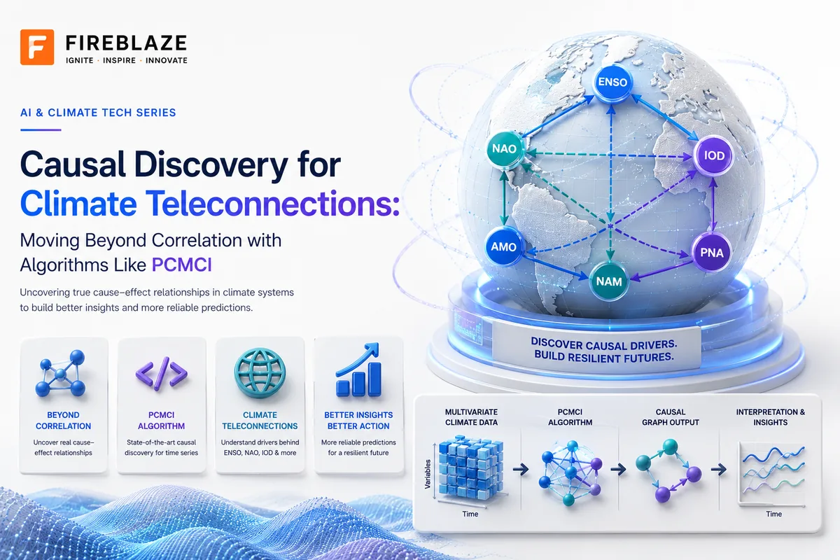
A domain-knowledge piece on why "which features mattered" — the SHAP/attribution question this series has covered so far — is not the same question as "what causes what, at what lag, through which pathway" — and why PCMCI, a specific causal discovery algorithm built for exactly this problem, is the tool that answers the second question instead of a fancier way of answering the first.

1. Hook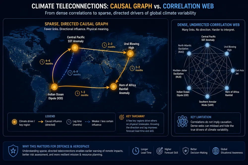

Every attribution method covered so far in this series — SHAP values, feature importances, saliency maps — answers a version of the same question: given a trained predictive model, which inputs did it lean on most to produce this output? That's a genuinely useful question, but it's a question about a model's behavior, not about the world's behavior, and the two can diverge sharply. A model can assign high SHAP importance to Arctic sea ice extent when predicting a cold-air outbreak over Europe simply because sea ice extent is correlated with the actual driver — a stalled polar vortex — without sea ice extent causing the outbreak at all, or with the causal arrow running in a more complicated, lagged, indirect way than a snapshot attribution score can express. Climate teleconnections are exactly the domain where this gap bites hardest: variables like El Niño sea surface temperature, the Indian Ocean Dipole, and Arctic sea ice are all correlated with each other and with regional weather outcomes, often because they share upstream drivers or influence each other with time lags of weeks to months — which means a correlation matrix, or an attribution score computed on top of one, will routinely light up variables that have no direct causal effect at all. Causal discovery algorithms, and specifically PCMCI (Runge et al., 2019), were built to solve precisely this problem for climate data: not "which variables are associated," but "which variables directly cause which others, at what time lag, once every spurious and indirect pathway has been accounted for." This piece is about how PCMCI actually does that, and where it can and can't be trusted to be right.

2. Core Explanation

2.1 Why Correlation — and Correlation-Based Attribution — Fails on Climate Data Specifically

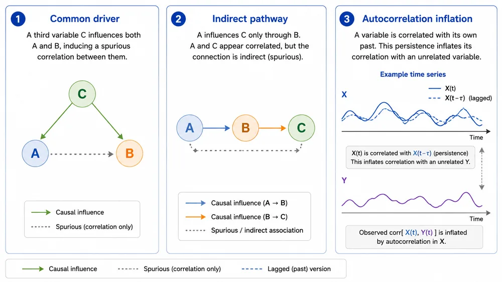
Three properties of Earth-system time series make naive correlation, and by extension correlation-flavored feature attribution, an unreliable guide to what's actually driving what:

Common drivers. Two climate variables can be strongly correlated purely because a third variable drives both of them. Central Pacific sea surface temperature and Indonesian rainfall can look connected in a correlation map when both are really being driven, at different lags, by the broader ENSO cycle — the correlation is real, but neither variable is causing the other.
Indirect pathways. A causal effect can pass through several intermediate variables before reaching its final target, and a raw correlation between the first and last variable in that chain looks identical to a direct causal link even though it isn't one.
Strong autocorrelation. Nearly every climate variable is strongly autocorrelated with its own recent past — today's sea surface temperature is a good predictor of tomorrow's mostly because of persistence, not because of anything else happening in the system. This inflates apparent correlations between any two persistent variables that happen to be evolving over similar timescales, whether or not one influences the other at all.

A domain-adapted causal discovery method has to explicitly correct for all three, not just compute cleverer correlations. This is precisely why PCMCI was built as an adaptation of a general-purpose causal discovery algorithm specifically to address strong autocorrelation in climate time series, rather than being a generic off-the-shelf method applied to Earth data without modification.

2.2 The PC Algorithm: The Foundation PCMCI Builds On

PCMCI's first building block is the PC algorithm, named after its inventors Peter Spirtes and Clark Glymour, a foundational method in the broader causal discovery literature for learning a causal graph structure from observational data. The core idea is conditional-independence testing: start by assuming every variable might causally affect every other variable, then iteratively test whether two variables are actually statistically independent once you condition on (control for) some subset of the other variables. If A and B become independent after conditioning on C, that's evidence C explains their apparent relationship — the direct A–B link gets removed from the graph. Repeating this test across all variable pairs and conditioning sets progressively prunes a fully connected, uninformative graph down to a sparse one that reflects actual direct dependencies.

Applied naively to climate time series, though, the PC algorithm runs into the autocorrelation and redundancy problems from Section 2.1 — conditioning on highly redundant neighboring time series decreases the apparent dependence between two remote locations, which lowers statistical power to detect real links, and datasets with hundreds or thousands of variables create serious computational problems for the PC algorithm on its own. This is the specific gap PCMCI closes.

2.3 What PCMCI Actually Does: Two Stages

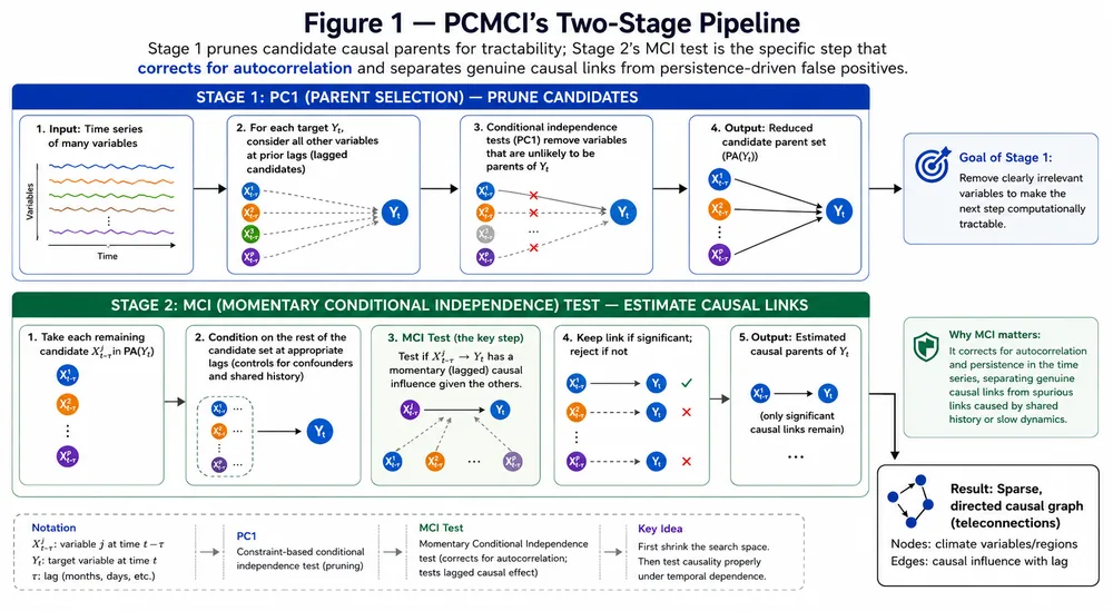
PCMCI is a two-step method: the first step finds the lagged "parents" (direct causal predecessors) of every variable using a PC-stable procedure, and the second step tests momentary conditional independence (MCI) to refine which of those candidate links are genuinely causal. It's worth unpacking both stages, since the second one is where PCMCI earns its name and its real advantage over plain PC:

Stage 1 — Condition selection (PC-stable): For every variable, PCMCI searches across time-lagged versions of all other variables and identifies a preliminary set of candidate causal "parents" — variables whose lagged values might directly influence it — while pruning away obviously irrelevant ones. This step controls the size of the conditioning sets that stage 2 will need to test, which is what keeps the method computationally tractable on large, high-dimensional climate datasets.
Stage 2 — Momentary Conditional Independence (MCI): For each remaining candidate link, PCMCI tests whether the specific lagged link between variable X at time t−τ and variable Y at time t remains statistically significant once conditioned on both variables' own separately identified parent sets. This specific conditioning choice is what corrects for the strong autocorrelation problem — by conditioning on each variable's own causal history in addition to the other candidate drivers, PCMCI distinguishes a link that reflects genuine new information transfer from a link that's really just two persistent, self-similar time series happening to move together.

The output is a causal adjacency structure — which variables causally affect which others, at which time lags — along with the strength of each identified relationship and a p-value for its statistical significance. A widely used extension, PCMCI+, adds the ability to detect contemporaneous (same-timestep) causal links in addition to lagged ones, which matters for fast-coupling atmospheric processes where cause and effect can appear within the same observation window used in the data.

2.4 A Worked Pathway: El Niño and Regional Drought, Stated the Way PCMCI States It

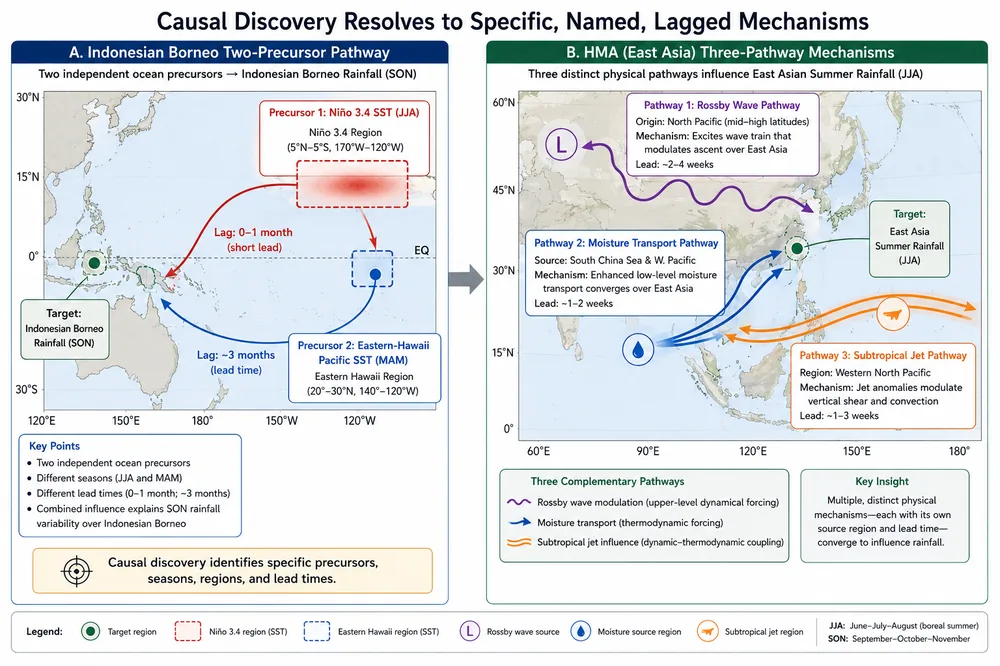
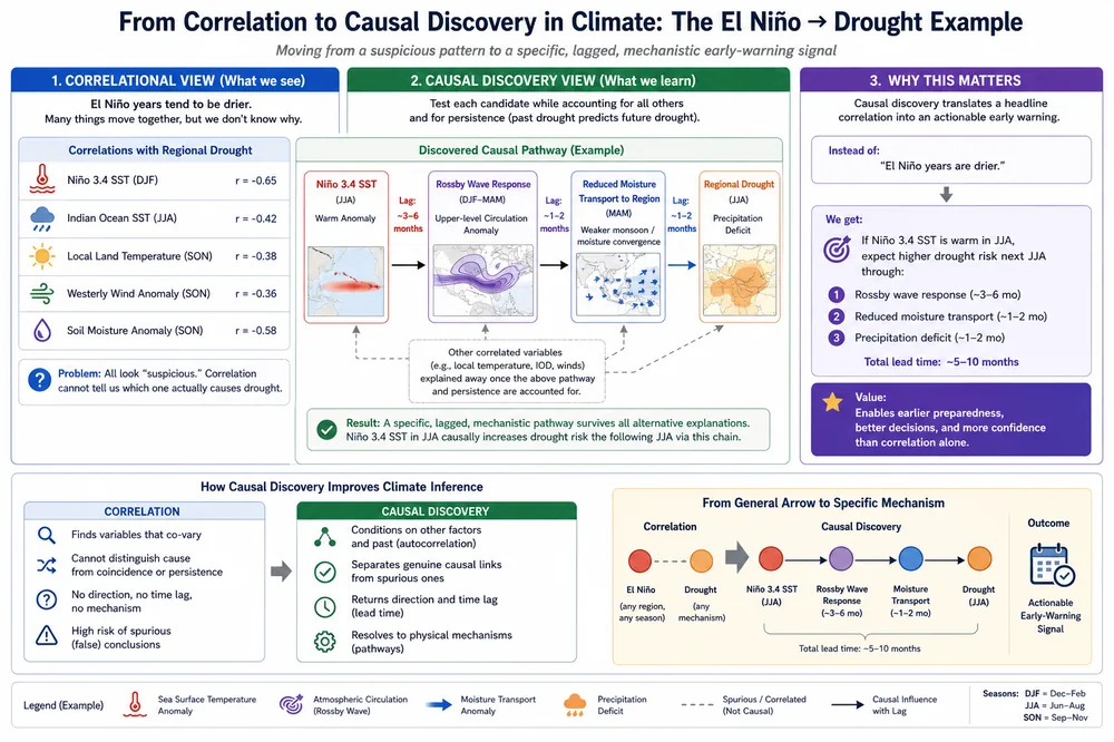
This is the point where it's worth being concrete rather than staying abstract, because "El Niño causes drought" is a correlational headline that PCMCI-style analysis actually breaks down into something more specific and more useful. Applied to Indonesian Borneo, a causal-network approach identified two distinct drivers of June–July–August drought rather than one vague "El Niño effect": Niño 3.4 sea surface temperature during the same June–July–August window (the core ENSO signal), and a separate sea surface temperature anomaly east of Hawaii in the preceding March–April–May, with the latter giving a three-month lead time for drought prediction based on its causal association. That's a materially different, more actionable statement than "SST correlates with drought" — it names a specific precursor region, a specific lag, and a specific downstream target.

A similar pattern shows up in work on high-mountain Asia precipitation, where researchers didn't just ask "does ENSO affect HMA rainfall" but used PCMCI+ to test three distinct, physically reasoned teleconnection pathways by which ENSO could plausibly influence the region — an extratropical Rossby wave response, tropical moisture transport from the Indian Ocean, and modulation of the subtropical westerly jet — and found that different pathways dominate in different months: November precipitation is modulated through the Rossby wave and moisture-transport pathways, while March precipitation runs primarily through the subtropical jet. That's the actual payoff of causal discovery over correlation in this domain: not just confirming that a relationship exists, but resolving which specific physical mechanism carries it, which is exactly the kind of detail a downstream risk or planning system needs and a correlation coefficient can't supply.

2.5 Beyond ENSO: Where Else PCMCI Has Actually Been Validated

El Niño–drought is the most intuitive example, but it's worth showing the method's range, since a single case study can look like a cherry-pick:

Stratospheric polar vortex prediction. Kretschmer et al. (2017) used causal-network precursor detection to identify tropospheric signals — including a characteristic high-pressure pattern over the Ural region — that precede extreme weakening of the stratospheric polar vortex, and a linear regression model built on these causal precursors correctly predicted 46% of extremely weak polar vortex states at lead times of 16 to 30 days, meaningfully extending on prior empirical prediction skill that had been limited to roughly 20 days.
Arctic sea ice and midlatitude winter circulation. An earlier causal-network method (a direct predecessor to PCMCI) applied to Arctic winter circulation data identified Barents and Kara sea ice as important drivers of tropospheric winter circulation, providing further confirmation of a proposed troposphere-stratosphere coupling pathway that had previously only been argued from correlation and physical reasoning.
Climate model evaluation. Rather than using causal discovery to study the real atmosphere, one line of work runs PCMCI on the output of CMIP6 climate models themselves and compares the resulting causal networks to the one recovered from reanalysis data — causal discovery methods are explicitly built to remove spurious links from common drivers and indirect pathways, and PCMCI has been tested extensively to successfully recover known interactions such as the tropical Walker circulation and predictors of polar vortex states — turning "does this climate model get its teleconnections right" into a checkable, graph-comparison question rather than a qualitative judgment call.
U.S. flash drought and Ethiopian drought. More recent applications have used PCMCI+ to search for remote sea-surface-temperature drivers of flash drought predictability over the continental U.S. at multi-week lead times, and separately, applying PCMCI to Ethiopian drought found the strongest causal association came from a sea-surface-temperature pattern with a twelve-month lag, dominated by the ENSO region of the Pacific — a genuinely long lead time a simple correlation screen at shorter windows would likely have missed.

2.6 Direct Contrast: PCMCI vs. SHAP/Attribution (Where This Series Started)

Since this piece is explicitly framed as moving past the attribution methods covered earlier in the series, the contrast is worth stating as a table rather than leaving it implicit:

Dimension	SHAP / Feature Attribution	PCMCI / Causal Discovery
What it operates on	A trained predictive model's input-output behavior	Raw observational time series directly — no predictive model required
What the output means	How much each input feature contributed to this model's prediction	Which variables actually causally influence which others, and at what lag, in the underlying system
Handles confounding?	No — a feature correlated with the true cause can receive high importance even with no causal role	Yes, by design — conditioning on other variables' parent sets is specifically how confounded and indirect links get pruned out
Handles time lags explicitly?	Only if lagged features were manually engineered as separate model inputs	Yes, natively — lag is a first-class output of the algorithm, not something that has to be hand-built into the feature set
What a "wrong" answer looks like	High importance assigned to a proxy variable that the model leaned on but that has no real-world causal role	A false-positive edge in the causal graph — usually from a violated assumption (see Section 2.7), not from model-fitting artifacts
Best use	Explaining and debugging a specific trained model's decisions	Building a mechanistic understanding of the system itself, independent of any one downstream model

The one-line version: SHAP tells you what a model paid attention to; PCMCI tells you what the climate system actually does. A variable can score high on the first and have zero role in the second, and conversely a variable with a real, well-established causal role can be underweighted by a model (and therefore by SHAP) if a correlated proxy was more convenient for that particular model to use.

2.7 A Caveat Worth Taking Seriously: The Assumptions Underneath "Causal"

This is the section that keeps this piece honest rather than turning "causal discovery" into a magic word. PCMCI's output is only interpretable as genuinely causal under three explicit assumptions, and all three can fail in real climate applications:

Causal sufficiency — the assumption that all common causes of the measured variables are themselves among the measured variables. If an unmeasured driver influences two of your input variables, PCMCI has no way to know that and may report a spurious direct link between them.
Causal Markov condition — the assumption that, given a variable's true causal parents, it's statistically independent of everything else in the system. This is a standard assumption in graphical causal modeling, not something PCMCI can verify from the data itself.
Faithfulness — the assumption that every conditional independence visible in the data reflects the true causal graph structure, rather than arising from a coincidental cancellation of effects.

Researchers working directly with these methods are explicit that the results depend on these assumptions holding: work on flood-driver causal discovery notes that prior knowledge of the physical system and relevant variables at appropriate timescales is required for applying PCMCI+ responsibly, and applications to global warming's effect on the polar vortex are described by their own authors as tools to quantify hypothesized causal pathways and test their consistency with the data, rather than to prove causality outright. That distinction — "consistent with a causal hypothesis" versus "proven causal" — is the honest framing PCMCI output actually supports. Practically, this means: which variables you decide to include in the analysis (driven by domain physical reasoning, not the algorithm) is doing real work in determining what the algorithm can and can't discover, and a PCMCI graph built on an incomplete variable set can still contain confounded, spurious edges — just fewer of them than a raw correlation matrix would.

2.8 Common Pitfalls

Treating a PCMCI edge as unconditional proof of causation. As Section 2.7 lays out, every edge in the output graph is conditional on causal sufficiency, the Markov condition, and faithfulness holding — none of which the algorithm can verify on its own from the data.
Skipping domain-driven variable selection. PCMCI's causal sufficiency assumption means omitting a real common driver from the input variable set is a direct route to a spurious edge between two of its effects — this is a modeling choice made by the analyst, not a limitation the algorithm can compensate for automatically.
Confusing "causal discovery" with "causal proof at the mechanism level." As the polar-vortex/global-warming causal-network application makes explicit, the right framing for most published climate applications is testing whether data is consistent with a hypothesized pathway, not manufacturing certainty from scratch.
Assuming SHAP and PCMCI answer the same question and can substitute for each other. Section 2.6 exists specifically to head this off — a feature mattering to a model's predictions and a variable causally driving the real system are related but genuinely different claims, and conflating them is the most common way attribution results get over-interpreted in a climate context.

3. Worked Example / Analogy

Picture a hospital investigating why patients on a particular ward keep spiking fevers at roughly the same time each evening. A purely correlational approach would flag everything that moves together with the fever spikes: the evening nurse shift change correlates with it, dinner service correlates with it, a nearby construction site's noise level correlates with it, because all of these also happen to cluster around the same time of day. A causal-discovery-style investigation does something different: it asks, for each candidate factor, "does this still predict the fever spike once I account for everything else that's also happening at that time, including the fact that fevers earlier in the day predict fevers later in the day?" Working through that conditioning, it turns out the nurse shift change and dinner service are both driven by the same underlying cause — hospital scheduling — and neither directly affects fever; but a specific medication administered during the shift change does have a genuine, lagged causal effect, showing up roughly ninety minutes after administration regardless of which nurse gives it or what time dinner arrives. The correlational approach would have handed investigators three equally "suspicious" candidates and no way to rank them; the causal-discovery approach hands them one specific mechanism, with a specific time lag, that survives once every alternative explanation has been tested and ruled out. El Niño and regional drought works exactly the same way: the correlational headline is "El Niño years are drier," but the causal-discovery answer specifies which sea-surface-temperature region, in which preceding season, driving drought through which physical pathway, months in advance — the difference between a suspicious pattern and an actionable, mechanistically grounded early-warning signal.

4. Application to Defence & Aerospace

For a Defence & Aerospace AI Centre of Excellence building risk-assessment and early-warning capability on top of a climate digital twin, the correlation-versus-causation distinction covered in this piece is not academic hair-splitting — it determines whether an early-warning signal is trustworthy enough to act on months in advance or is a coincidental pattern that will quietly fail the first time the underlying confounder shifts. A purely correlational drought or extreme-weather early-warning system built on SHAP-style attribution over a predictive model inherits every one of that model's spurious associations; a PCMCI-derived causal graph, subject to the assumptions in Section 2.7, gives planners something closer to a genuine mechanistic precursor with an associated lead time — the Indonesian Borneo case (a three-month lead from a named precursor region) and the polar-vortex case (16–30 day lead, 46% detection skill on extreme states) are both directly the kind of lead time that matters for pre-positioning humanitarian logistics, adjusting basing and flight-operations risk postures ahead of stratospheric-driven cold outbreaks, or flagging regions where a known causal drought pathway is entering its precursor phase. The Section 2.7 caveat is the operational discipline that has to travel with any of this: a causal graph built on an incomplete variable set, or applied outside the physical regime it was validated in, can still produce a confident-looking but spurious early-warning trigger — which is exactly why the honest framing from the climate-science literature itself ("consistent with a hypothesized pathway," not "proven") is the correct standard to carry into a decision-support system rather than quietly upgrading it to certainty along the way.

5. Quick-Reference Glossary

Term	Meaning
Teleconnection	A statistical or causal link between climate anomalies in two widely separated geographic regions (e.g., Central Pacific sea surface temperature and Indonesian rainfall)
Causal discovery	A family of algorithms that infer the causal structure — which variables directly influence which others, and how — from observational data, rather than assuming or hand-specifying it
PC algorithm	The foundational conditional-independence-based causal discovery method (Spirtes & Glymour) that PCMCI builds on and adapts for time series
PCMCI	"PC + Momentary Conditional Independence" — a two-stage causal discovery algorithm (Runge et al., 2019) adapted specifically for high-dimensional, autocorrelated climate time series
Momentary Conditional Independence (MCI)	PCMCI's second-stage test, which conditions on both variables' own separately identified causal parents to correct for autocorrelation-driven false positives
Confounder / common driver	A variable that causally influences two other variables, making them appear correlated (or causally linked) with each other even though neither directly causes the other
Causal sufficiency	The assumption that all common causes of the measured variables are themselves included among the measured variables — a key limitation when unmeasured drivers exist
Lagged vs. contemporaneous link	A lagged causal link connects a cause at an earlier timestep to an effect later on; a contemporaneous link connects variables within the same observation window (handled by the PCMCI+ extension)
Causal Effect Network (CEN)	An earlier causal-network method, closely related to and a direct predecessor of PCMCI, used in several of the Arctic-teleconnection studies referenced above