Linear Regression Algorithm in Machine Learning Explained

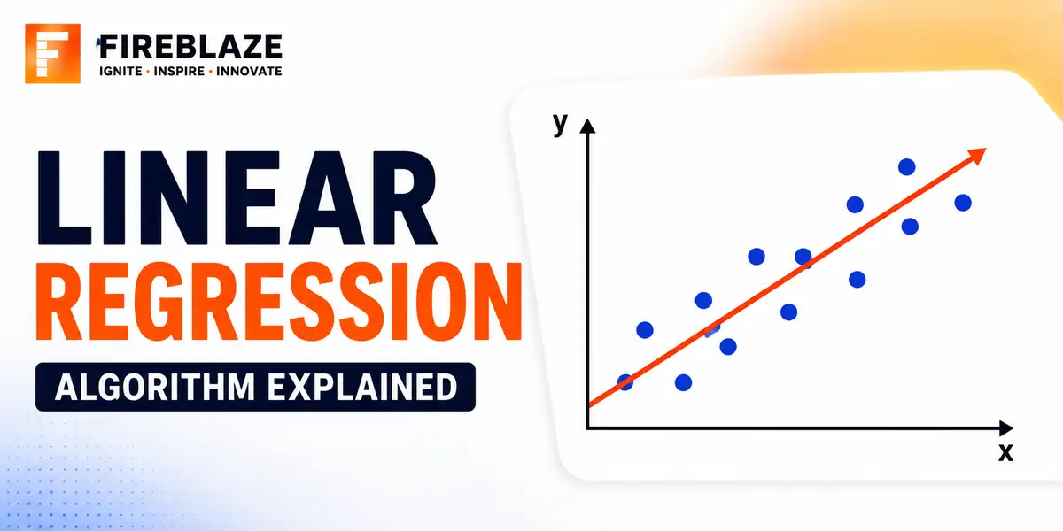
Quick answer: Learn linear regression including the equation, assumptions, cost function, gradient descent, model evaluation metrics, and common interview questions.

What is Linear Regression?

Linear regression models the relationship between one or more input features and a continuous target variable by fitting a straight line, or a flat plane in higher dimensions, that best predicts the target from the inputs.

The Linear Regression Equation

y = b0 + b1*x1 + b2*x2 + ... + bn*xn

Where y is the predicted value, b0 is the intercept, and each b coefficient represents how much y changes for a one-unit increase in that specific feature, holding the others constant.

A Simple Example in Python

from sklearn.linear_model import LinearRegression
import pandas as pd

X = df[['square_feet', 'num_bedrooms']]
y = df['price']

model = LinearRegression()
model.fit(X, y)

print(model.intercept_)   # b0
print(model.coef_)        # [b1, b2]

The Cost Function: Minimising Error

Linear regression finds the coefficients that minimise the Mean Squared Error, the average squared difference between predicted and actual values, across all training examples.

MSE = (1/n) * Σ(actual - predicted)²

How Gradient Descent Finds the Best Fit

Gradient descent iteratively adjusts the coefficients in the direction that reduces the cost function, taking small steps controlled by a learning rate, until the error stops meaningfully decreasing. For simple linear regression, an exact closed-form solution also exists and is what Scikit-Learn uses by default, but gradient descent becomes necessary for very large datasets or more complex models.

Key Assumptions of Linear Regression

• Linearity: the relationship between features and target is genuinely linear

• Independence: observations are independent of each other

• Homoscedasticity: the variance of errors is roughly constant across all predicted values

• Normality of residuals: prediction errors are approximately normally distributed

• No severe multicollinearity: input features are not too strongly correlated with each other

Evaluating a Linear Regression Model

from sklearn.metrics import mean_squared_error, r2_score

predictions = model.predict(X_test)
print("RMSE:", mean_squared_error(y_test, predictions, squared=False))
print("R-squared:", r2_score(y_test, predictions))

R-squared indicates what proportion of the variance in the target the model explains, ranging from 0 to 1, where higher is generally better, though a very high value can also be a sign of overfitting.

Why Multicollinearity Matters

When two input features are highly correlated with each other, the model struggles to separate their individual effects, making coefficients unstable and hard to interpret, even though the model's overall predictive accuracy may be barely affected.

Common Interview Questions

What does the R-squared value actually tell you?

It represents the proportion of variance in the target variable that the model explains. An R-squared of 0.8 means the model explains 80 percent of the variability in the outcome.

What happens if the linearity assumption is violated?

The model will systematically underfit the true relationship, and a transformation of the features, or a different, non-linear model, is usually needed instead.