Remaining Useful Life 101: How Predictive Maintenance Models Actually Work

Remaining Useful Life 101: How Predictive Maintenance Models Actually Work
Part of our GenAI-Augmented Predictive Maintenance for Jet Engines series — the technical foundation every RUL model, generative augmentation technique, and maintenance-scheduling system in this series is ultimately built on.
1. Hook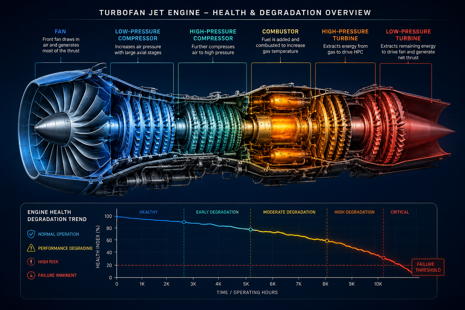
A commercial turbofan engine costs anywhere from $10 million to over $40 million, generates a maintenance event roughly every few thousand flight hours, and — if it fails unexpectedly rather than on a planned schedule — can ground an aircraft, cascade delays across an airline's entire network, and in the worst case, threaten flight safety. The entire predictive-maintenance industry exists to answer one deceptively simple question about that engine: how many more cycles does it have left before it needs to come off-wing? Getting that number right, and understanding exactly how models arrive at it, is the foundation everything else in modern aviation maintenance AI is built on — and almost none of the popular explanations of "predictive maintenance" actually walk through how the number is calculated.
2. Core Explanation
2.1 What "Remaining Useful Life" Actually Means
Remaining Useful Life (RUL) is defined as the number of operational cycles (or, in some formulations, flight hours) a piece of equipment can continue to function within acceptable performance and safety limits before it requires maintenance or replacement. The word "cycle" here has a specific engineering meaning for a jet engine: one cycle is typically one full flight — from engine start, through takeoff, cruise, and descent, to shutdown — because the thermal and mechanical stress an engine experiences follows this start-stop pattern far more than it follows raw elapsed time.
This distinction matters enormously for how RUL is modeled. A engine that flies twelve short regional hops a day accumulates cycles (and the associated thermal stress of repeated startup and shutdown) far faster than an engine on a single long-haul route, even if both log similar total flight hours in a month. Any RUL model that ignores this and treats "hours" and "cycles" as interchangeable will systematically mis-predict degradation for short-haul fleets — a subtlety that trips up a surprising number of introductory tutorials on this topic.
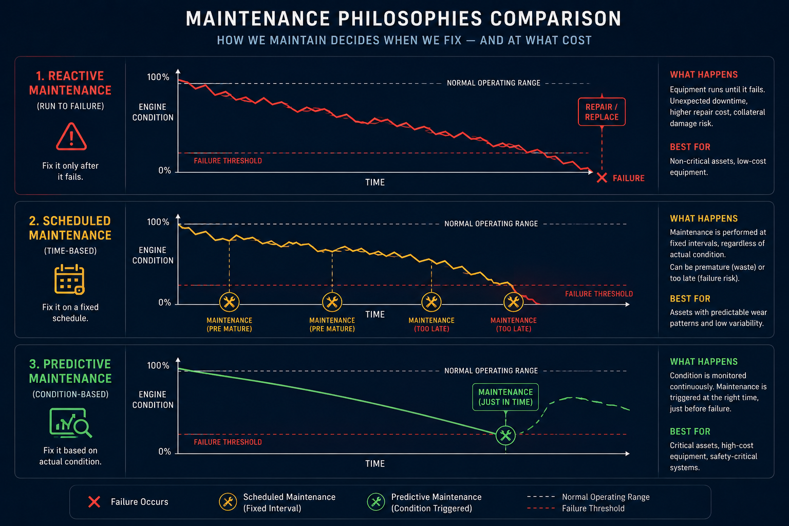
RUL prediction sits within the broader discipline of Prognostics and Health Management (PHM), which itself sits downstream of two earlier maintenance philosophies worth naming explicitly, because the contrast explains why RUL modeling is valuable in the first place:
- Reactive (run-to-failure) maintenance — fix or replace only after something breaks. Cheapest per-event, but catastrophically expensive and dangerous when the "something" is a jet engine mid-flight.
- Scheduled (preventive) maintenance — replace or service components at fixed calendar or cycle intervals regardless of actual condition, based on statistical failure rates across a fleet. Safer than reactive maintenance, but wasteful — most components removed under a fixed schedule still have substantial useful life left in them.
- Predictive (condition-based) maintenance — use the equipment's actual, observed degradation state to decide when maintenance is needed, ideally just before failure rather than on an arbitrary calendar date. RUL prediction is the mathematical engine that makes this third approach possible.
2.2 What's Actually Degrading Inside a Turbofan Engine
Before looking at how RUL is modeled statistically, it helps to understand what's physically happening inside the machine, because the sensor data used for RUL prediction is measuring the downstream signature of these physical processes, not the processes themselves.
A modern turbofan engine is built around a sequence of rotating stages: a fan, a low-pressure compressor (LPC), a high-pressure compressor (HPC), a combustor, a high-pressure turbine (HPT), and a low-pressure turbine (LPT). Air is compressed progressively through the fan and compressor stages, mixed with fuel and ignited in the combustor, and the resulting hot expanding gas drives the turbine stages, which in turn power the compressors and fan through a shared shaft.
Degradation in this system shows up as a handful of physical mechanisms, each with a distinct sensor signature:
- Compressor and turbine blade erosion and fouling — dust, debris, and thermal cycling gradually erode blade surfaces and allow small performance-robbing gaps to form, reducing compression efficiency.
- Seal and clearance degradation — components that should fit tightly gradually loosen with thermal cycling and vibration, allowing gas to leak past stages it should be doing work in, which shows up as pressure and efficiency sensor drift.
- Thermal fatigue in hot-section components — the combustor and turbine stages operate at extreme temperatures, and repeated heating/cooling cycles (i.e., repeated flight cycles, not just elapsed hours) cause microscopic material fatigue that accumulates irreversibly.
Crucially, none of these mechanisms are usually observed directly — instead, a bank of sensors (in the standard NASA C-MAPSS benchmark dataset, twenty-one of them, covering temperatures, pressures, and rotational speeds at various stages) captures the downstream effect of this degradation: rising exhaust gas temperature for a given thrust setting, falling compressor efficiency, shifting rotational speeds needed to maintain the same output. RUL modeling is, at its core, the task of learning the mapping between these indirect sensor signatures and the underlying, unobserved wear state of the machine.
2.3 The Benchmark Everyone Uses: NASA's C-MAPSS Dataset
Almost every publicly available RUL research paper, tutorial, and Kaggle project benchmarks against the same dataset: the NASA Turbofan Engine Degradation Simulation dataset, generated using a NASA tool called C-MAPSS (Commercial Modular Aero-Propulsion System Simulation), originally released alongside the 2008 PHM (Prognostics and Health Management) Society data challenge. Understanding its structure well is essential, because nearly every modeling choice discussed later in this piece — and every project in this series — is shaped by how this dataset is built.
C-MAPSS provides simulated run-to-failure trajectories: each "engine unit" in the dataset starts in a healthy state with some unknown, randomized initial wear, operates normally for a period, begins degrading at some point, and continues degrading until it crosses a failure threshold. Every row in the dataset records one operational cycle for one engine unit, and contains an engine ID, the cycle number, three operational settings (altitude, Mach number, and throttle resolver angle — together defining the flight regime the engine was operating under for that cycle), and readings from 21 onboard sensors covering temperatures, pressures, and shaft speeds at different stages of the engine.
The dataset is split into four subsets of increasing difficulty, distinguished by how many operating conditions and failure modes each one contains:
| Subset | Operating Conditions | Fault Modes | Approx. Training Engines | Difficulty |
|---|---|---|---|---|
| FD001 | 1 | 1 | 100 | Baseline — single flight regime, single degradation pattern |
| FD002 | 6 | 1 | ~260 | Harder — engine must generalize across six distinct operating regimes |
| FD003 | 1 | 2 | 100 | Harder — single regime, but two distinct ways the engine can fail |
| FD004 | 6 | 2 | ~248 | Hardest — six operating regimes and two fault modes simultaneously |
(Note: some published sources report slightly different exact engine counts for FD002/FD004 — figures in the low-to-mid 200s to high-200s range depending on the specific release — so treat the counts above as approximate and verify against your specific downloaded copy before citing exact numbers in a paper.)
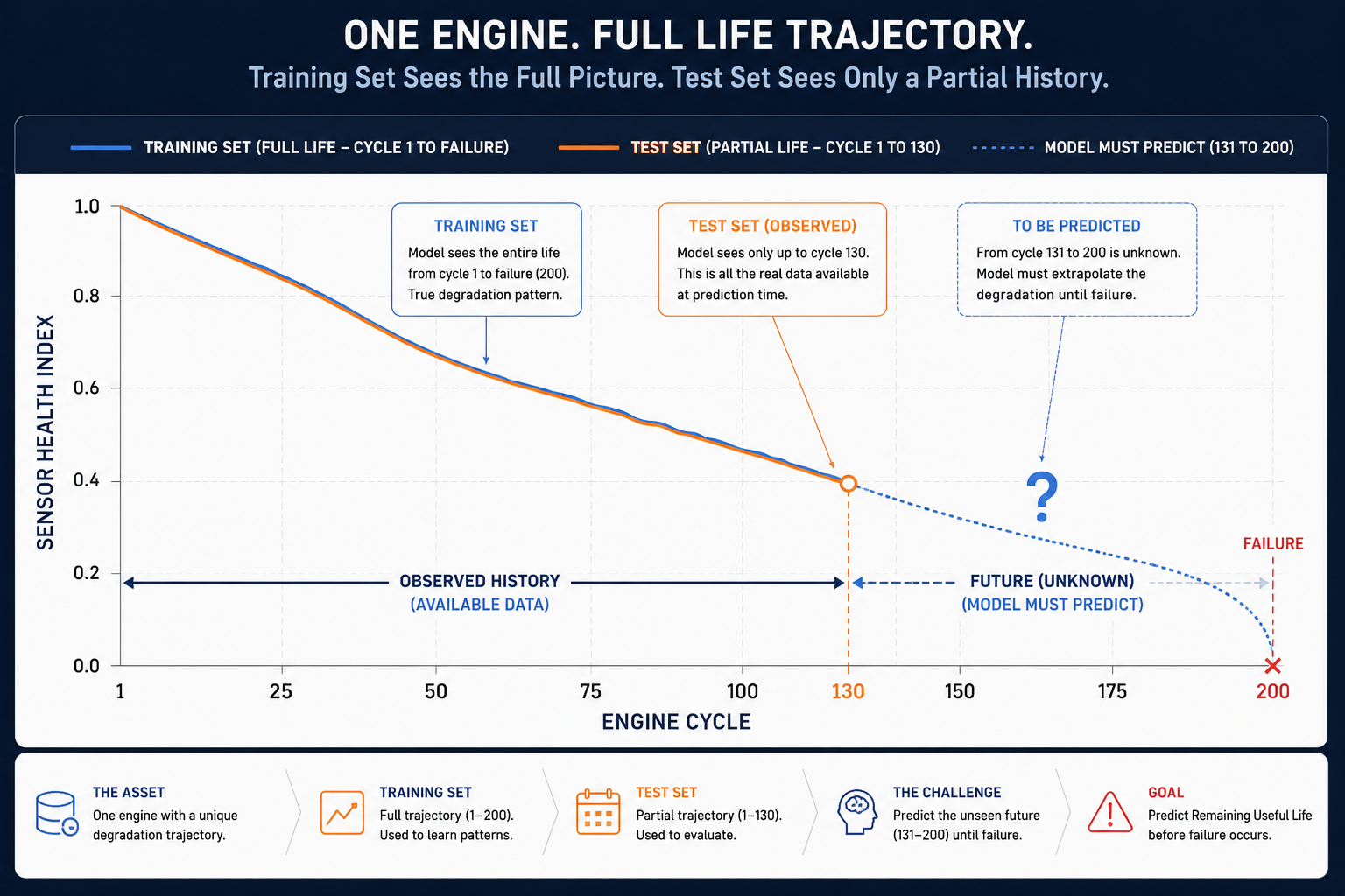
Two features of this dataset are worth calling out because they shape every modeling decision downstream: first, seven of the twenty-one sensors are essentially constant throughout the engine's life and carry little to no degradation signal, so most published approaches drop them and work with the remaining fourteen active sensors. Second, and more subtly, the training and test sets are constructed differently on purpose: training trajectories run all the way to failure (so the true RUL at every cycle is simply "cycles remaining until the trajectory ends"), while test trajectories are deliberately truncated at some random point before failure — the model's job is to predict how many cycles remain beyond that truncation point, without ever having seen the engine actually fail. This train/test asymmetry is what makes C-MAPSS a genuine prognostics benchmark rather than a simple regression exercise: it forces a model to extrapolate a degradation trend into the future, not just fit a curve to data it can see.
2.4 From Raw Sensors to a Trainable Target: Health Indicators and the RUL Label
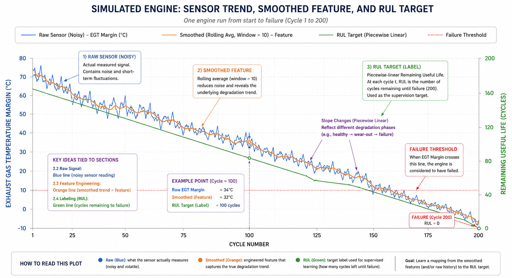
Raw sensor readings alone don't make a usable training target — a critical design decision has to be made about what the model is actually being asked to predict at each cycle, and this decision has a name worth knowing: the piecewise-linear RUL target.
Here's the problem it solves. If you simply label every cycle with "true cycles remaining until failure" (a straight linear countdown from the first cycle), you're implicitly telling the model that an engine's condition is already declining meaningfully from cycle one — which is physically false. Real engines operate in a genuinely healthy, roughly constant-performance state for a large portion of their life, and only start exhibiting a measurable degradation trend in the later portion of their lifespan. To reflect this, the overwhelming majority of published C-MAPSS approaches cap the RUL label at a constant value (commonly 125 or 130 cycles) for all early cycles, and only let the label count down linearly once the engine enters its true degradation phase. This produces a target curve that's flat for most of an engine's early life, then linearly decreasing toward zero as failure approaches — matching the actual physical behavior far better than a naive straight-line countdown, and it measurably improves model training in nearly every published comparison that tests both approaches.
Beyond the label itself, feature engineering typically layers on top of the raw 14 active sensors:
- Rolling statistics (moving averages, moving standard deviations) over a short window of recent cycles, to smooth out sensor noise while preserving the underlying trend.
- Rate-of-change features — the first derivative of key sensors cycle-over-cycle, which often carries an earlier and clearer degradation signal than the raw sensor level itself.
- Health indices — engineered composite scores (sometimes built via principal component analysis or simple weighted combinations) that compress the fourteen active sensors into one or two dimensions summarizing overall engine health, which is especially useful for visualization and for simpler downstream models.
- Operating-condition normalization — for the multi-condition subsets (FD002, FD004), sensor readings must be normalized within each of the six operating regimes before they're comparable across cycles, since a "normal" pressure reading at cruise altitude looks nothing like a "normal" reading at takeoff thrust — conflating the two without normalization is one of the most common beginner mistakes on this dataset.
2.5 The Three Families of RUL Models — And Why They're Not Interchangeable
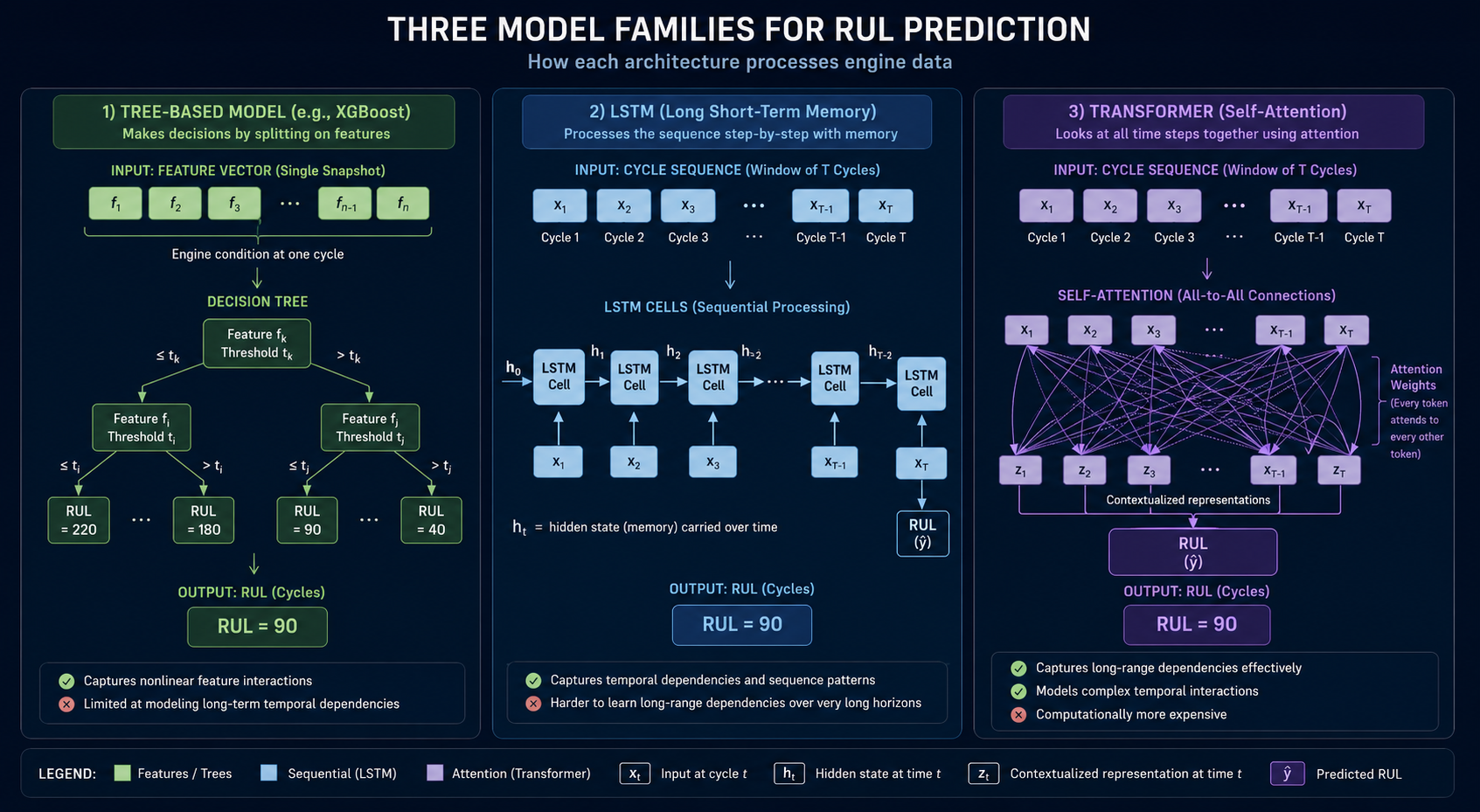
With a properly engineered target and feature set in hand, three broad families of modeling approaches dominate the published literature and practical toolkits, each with a genuinely different underlying assumption about the degradation process.
Traditional machine learning regressors — gradient-boosted trees (XGBoost, LightGBM, CatBoost), random forests, and support vector regression — treat each cycle (or each engineered feature window) as an independent row and predict RUL directly from the current feature vector. These models are fast to train, require comparatively little data, and are highly interpretable via feature importance, but they have no inherent memory of the sequence — they don't natively know that cycle 150 came after cycle 149 unless that history is manually engineered into the feature set via rolling windows.
Recurrent sequence models — chiefly Long Short-Term Memory (LSTM) networks and their bidirectional variants — process the sensor sequence step by step, maintaining an internal memory state that carries forward the trajectory's recent history. This makes them a natural fit for RUL prediction, since degradation is fundamentally a temporal, trending process, and an LSTM can in principle learn what a "worsening trend" looks like rather than needing that trend hand-engineered into rolling-window features. The cost is a larger data and compute requirement, more careful hyperparameter tuning (particularly the sequence window length fed into the network), and materially lower interpretability than a tree-based model.
Transformer-based models, adapted from natural language processing, have increasingly been applied to RUL prediction over the past several years. Their self-attention mechanism lets the model weigh the relevance of every prior cycle in the input window when forming a prediction, rather than propagating information step-by-step through a recurrent memory cell the way an LSTM does — in principle allowing them to capture longer-range dependencies more directly. In practice, transformer-based RUL models tend to need larger training sets and more careful regularization to avoid overfitting on a dataset with only a few hundred training trajectories, which is part of why gradient-boosted trees and LSTMs remain the more common baseline choices in published C-MAPSS benchmarks even as transformer architectures gain ground in the research literature.
| Model Family | Core Mechanism | Strength | Weakness | Typical Use Case |
|---|---|---|---|---|
| Gradient-boosted trees / classical ML | Feature-vector regression, no native sequence memory | Fast, interpretable, data-efficient | Needs manual feature engineering to capture trends | Fast baselines, production systems needing explainability |
| LSTM (recurrent) | Sequential processing with internal memory state | Learns temporal trends natively | Slower to train, less interpretable, sequence-length tuning needed | The most common deep-learning baseline in C-MAPSS literature |
| Transformer | Self-attention across the full input window | Captures long-range dependencies flexibly | Data-hungry, prone to overfitting on small trajectory counts | Research frontier; growing adoption as datasets and compute scale |
2.6 How These Models Are Actually Scored — And Why RMSE Alone Is Misleading
Here is the detail almost every introductory tutorial on this topic skips, and it matters enormously for anyone building or evaluating a real RUL model: the standard regression metric, RMSE (Root Mean Squared Error), treats early and late prediction errors as equally bad — but in a maintenance context, they are not.
RMSE is calculated in the usual way — the square root of the mean of squared prediction errors across all test samples — and it's genuinely useful as a general-purpose accuracy summary. But it's symmetric: a prediction that's 10 cycles too early (predicting the engine has less life left than it actually does, which just means slightly premature, safe maintenance) contributes exactly the same penalty as a prediction that's 10 cycles too late (predicting the engine has more life left than it actually does, which risks an in-service failure). Anyone who has thought for more than a few seconds about the actual cost asymmetry of these two error types can see why treating them identically is a poor fit for a safety-critical maintenance decision.
This is precisely why the original PHM08 data challenge introduced an asymmetric scoring function, which has since become the standard companion metric alongside RMSE in essentially all serious C-MAPSS research. It's defined as an exponential penalty that grows much faster for late predictions than for early ones:
For early prediction (di < 0):
si = exp(-di/13) - 1
For late prediction (di ≥ 0):
si = exp(di/10) - 1
where d_i is the prediction error (predicted RUL minus true RUL) for sample i, and the total score is the sum of s_i across all test samples. Notice the two scaling constants: 13 for early predictions, 10 for late ones — the smaller denominator on the late-prediction branch means the exponential penalty ramps up faster per cycle of lateness than per cycle of earliness, exactly encoding the "a surprise failure is worse than a slightly-too-early maintenance visit" intuition into the evaluation metric itself.
This has a very practical consequence for model selection: two models can have nearly identical RMSE while having dramatically different PHM08 scores, because RMSE can't see which direction the errors point in. A model whose errors skew slightly early will look similar to, or even worse than, a model whose errors skew slightly late under RMSE — but the second model is meaningfully more dangerous in an operational maintenance context, and only the asymmetric score reveals this. Published benchmarks on FD001 with strong models typically report RMSE in roughly the 12–15 cycle range alongside scores in the low-to-mid hundreds, though both figures vary considerably across papers depending on architecture, feature engineering, and exactly how the piecewise RUL label was constructed — treat any single reported number in the literature as one data point in a fairly wide, method-dependent range rather than a fixed ceiling.
| Metric | Formula Intuition | Penalizes Late Predictions More? | What It's Good For |
|---|---|---|---|
| RMSE | Square root of mean squared error | No — symmetric | General accuracy comparison, familiar to any ML practitioner |
| PHM08 Score | Asymmetric exponential penalty (steeper for late predictions) | Yes | Operationally realistic comparison; the metric that actually reflects maintenance risk |
2.7 Why This Is Genuinely Harder Than a Standard Regression Problem
It's worth being explicit about why RUL prediction resists being treated as "just another regression task," because underestimating this is where a lot of otherwise-competent data science goes wrong on this dataset.
First, the test-set truncation described in Section 2.3 means the model is always extrapolating, never interpolating — it's being asked to predict beyond the last observed data point, into territory it has no direct sensor evidence for, based purely on the trend established so far. This is a fundamentally harder task than standard regression, where test points typically fall within the same distribution the model was trained on.
Second, degradation trajectories vary significantly between individual engine units even under identical nominal operating conditions, because of manufacturing variation and unknown initial wear — meaning the model has to learn a general degradation pattern robust enough to apply to a specific unit whose exact starting condition it never directly observes.
Third, and this is the direct throughline to the rest of this series, catastrophic, severe-degradation trajectories are inherently underrepresented in any real or simulated fleet dataset — precisely because engines are designed, and generally succeed, at not failing catastrophically very often. A model trained predominantly on "typical" gradual degradation patterns tends to underperform specifically on the rare, severe cases that matter most operationally — which is exactly the gap our companion piece in this series (on generative data augmentation for rare failure modes) is built to address.
2.8 From Simulation to Real Fleet Data — Where C-MAPSS Simplifies Reality
It's worth being honest about something most tutorials gloss over entirely: C-MAPSS is a simulation, not flight-recorder data pulled from a real airline or military fleet, and the gap between the two matters if you're planning to take techniques validated on this benchmark and apply them operationally.
C-MAPSS trajectories are generated by a physics-based simulation model with injected sensor noise, which means every engine in the dataset degrades according to the same underlying simulated fault-progression physics, just with different randomized starting wear and randomized noise. Real fleet data is messier in ways that matter: sensors drift and get recalibrated or replaced mid-life, maintenance actions (component swaps, borescope inspections, on-wing washes) partially reset degradation in ways that aren't cleanly recorded in the sensor stream, and — critically — real fleets essentially never fly an engine to actual catastrophic failure, because operators pull engines for maintenance well before that point for obvious safety reasons. This means real-world RUL datasets are almost always right-censored: you know an engine was healthy up to the point of its last recorded maintenance action, but you don't have a clean, labeled "this is exactly cycle zero of remaining life" data point the way C-MAPSS's simulated failure threshold gives you for free.
This censoring problem is precisely why a parallel body of technique — survival analysis methods borrowed from biostatistics and reliability engineering (Kaplan-Meier estimators, Cox proportional hazards models, and their more recent deep-learning extensions like DeepSurv) — shows up frequently in real-world predictive maintenance work even though it's largely absent from C-MAPSS tutorials, since C-MAPSS conveniently sidesteps the censoring problem by simulating engines all the way to failure in its training set. Anyone moving from a C-MAPSS proof-of-concept toward a real fleet deployment should expect to spend meaningful engineering effort on exactly this gap — handling censored, maintenance-interrupted trajectories rather than clean run-to-failure sequences — before a benchmark-validated architecture translates into a production-ready system.
2.9 Common Pitfalls When Building an RUL Model
A handful of mistakes show up so frequently in beginner and even intermediate C-MAPSS projects that they deserve to be named explicitly, since avoiding them is often the difference between a benchmark-competitive result and a model that looks fine in a notebook but fails to generalize:
- Data leakage across the train/test split via global normalization. Computing mean and standard deviation for sensor normalization across the entire dataset — training and test combined — before splitting leaks information about the test distribution into the training process. Normalization statistics should be computed on the training set only, and then applied to the test set.
- Ignoring operating-condition clusters on FD002/FD004. As noted in Section 2.4, failing to normalize within each of the six operating regimes separately is one of the most common reasons a model that performs well on FD001 collapses in performance when applied to FD002 or FD004 — the raw sensor scale differences between regimes can dwarf the actual degradation signal if left unaddressed.
- Using a single train/test split without cross-validation across engine units. Because trajectories from the same engine unit are highly correlated cycle-to-cycle, a random row-level split (rather than splitting by whole engine unit) can leak near-identical cycles from the same trajectory into both train and test sets, producing an optimistic performance estimate that won't hold up on genuinely unseen engines.
- Reporting only RMSE and omitting the PHM08 score. As covered in Section 2.6, this alone can make an operationally worse (late-error-prone) model look equivalent to, or better than, a safer one.
- Treating the piecewise RUL cap (Section 2.4) as a fixed universal constant. The commonly cited value of 125–130 cycles is a convention adopted by most published work for comparability, not a physical law — the appropriate cap depends on the actual degradation-onset behavior of the specific fleet or dataset being modeled, and blindly reusing a published constant on a different engine family or dataset without re-examining it is a subtle source of avoidable error.
| Pitfall | Symptom | Fix |
|---|---|---|
| Global normalization leakage | Suspiciously strong validation performance that doesn't hold on new data | Fit normalization stats on training data only |
| Ignoring operating-condition clusters | Model works on FD001, collapses on FD002/FD004 | Normalize within each operating regime separately |
| Row-level rather than unit-level splitting | Overoptimistic cross-validation scores | Split by whole engine unit, never by individual row |
| RMSE-only reporting | Model looks fine on paper, riskier in practice | Always report the PHM08 asymmetric score alongside RMSE |
| Blindly reusing the 125-cycle RUL cap | Poor fit on a fleet with different degradation-onset timing | Re-derive the cap from the actual degradation-onset behavior of the target fleet |
3. Worked Example / Analogy
Think of RUL prediction like estimating how many more times you can use a pencil before it's too short to hold comfortably. You don't need to measure the exact remaining wood length precisely at every single moment — what you actually track is the rate at which it's shrinking: how many millimeters shorter it gets per day of use, whether that rate has been speeding up recently (maybe you've started sharpening it more aggressively), and how that trend compares to pencils you've used before down to the point where they became too short to hold.
Now imagine you're asked to make this prediction before the pencil has actually become too short — you're handed a pencil that's been used for a while and shown its wear pattern only up to the current moment, and asked "how many more sharpenings does this one have left?" That's exactly the structure of the C-MAPSS test set: you see the trend, but not the ending, and you have to extrapolate. And here's the part that maps directly onto the asymmetric scoring function: if you guess the pencil will last five more sharpenings when it actually lasts eight, that's a mildly wasteful early guess — you replace it a bit sooner than strictly necessary, no real harm done. But if you guess it'll last eight when it actually breaks after five, you're now holding a stub mid-sentence with no backup — a genuinely disruptive failure. RUL scoring is built to reflect that these two wrong guesses are not equally bad, even though they're the same "distance" from being right.
4. Application to Defense & Aerospace
For a Defense & Aerospace AI Center of Excellence, RUL modeling isn't just a Kaggle benchmark exercise — it maps directly onto fleet sustainment economics and, in military contexts, mission readiness. A military transport or fighter fleet's operational availability is directly gated by how many engines are in scheduled maintenance at any given time, and a fleet-wide shift from calendar-based to condition-based maintenance — the entire premise this section's dataset and modeling techniques exist to enable — can materially increase the number of aircraft available for tasking on any given day without adding a single new engine to the inventory.
The specific technical points covered above translate directly into defense procurement and engineering priorities: the cycle-versus-hours distinction (Section 2.1) matters enormously for military aircraft with highly variable mission profiles, where a single airframe might fly a mix of short training sorties and long-endurance missions in the same month; the asymmetric scoring logic (Section 2.6) maps directly onto mission-readiness risk tolerance, where an unexpected in-flight failure carries a categorically different cost than a slightly conservative early maintenance pull; and the extrapolation challenge (Section 2.7) is exactly why defense sustainment programs increasingly pair RUL models with the kind of generative rare-failure-mode augmentation and explainable maintenance-scheduling layers covered elsewhere in this series — a raw RUL number alone, without confidence bounds or an explanation a maintenance planner can act on, is operationally incomplete for a fleet where downtime has strategic, not just financial, cost.
5. Quick-Reference Glossary
| Term | Meaning |
|---|---|
| RUL | Remaining Useful Life — the number of cycles or hours a system can operate before requiring maintenance |
| PHM | Prognostics and Health Management — the broader engineering discipline RUL prediction belongs to |
| C-MAPSS | Commercial Modular Aero-Propulsion System Simulation — NASA's turbofan simulation tool behind the benchmark dataset |
| Cycle | One complete flight (start, takeoff, cruise, descent, shutdown) — the standard unit of accumulated engine stress |
| HPC / LPC | High-Pressure / Low-Pressure Compressor — engine stages that compress incoming air |
| HPT / LPT | High-Pressure / Low-Pressure Turbine — engine stages driven by combustion gas that power the compressors and fan |
| Piecewise-linear RUL target | The convention of capping the RUL label at a constant value during an engine's healthy phase, then counting down linearly once true degradation begins |
| RMSE | Root Mean Squared Error — a symmetric accuracy metric that penalizes early and late predictions equally |
| PHM08 Score | The asymmetric evaluation metric from the original 2008 data challenge, penalizing late predictions more heavily than early ones |
| Right-censoring | The real-world data condition where an engine's true failure point is never observed because it was pulled for maintenance beforehand |
| Survival analysis | A family of statistical methods (Kaplan-Meier, Cox proportional hazards) designed specifically to handle censored time-to-event data |
6. Further Reading
This piece is the technical foundation for the rest of our GenAI-Augmented Predictive Maintenance series. Continue with "Why Rare Failure Modes Break Predictive Maintenance Models (and How Synthetic Data Fixes It," which picks up directly from Section 2.7's extrapolation challenge, and our RUL-Predictor project blog, which walks through building and benchmarking exactly the kind of LSTM-based model described in Section 2.5 against the C-MAPSS dataset introduced here.